What is a Neural Network?

Neural networks are a class of machine learning algorithms inspired by the functioning of biological neurons. They are widely used in artificial intelligence for image recognition, natural language processing, time series forecasting, and many other fields. Thanks to their ability to model complex relationships in data, they have become one of the pillars of deep learning.

1 - Basic Structure of a Neural Network

1.1 - Neurons and Biological Inspiration

Neural networks are inspired by the way the human brain processes information. Each artificial neuron mimics a biological neuron, receiving inputs, applying a transformation, and passing the result to the next layer.

1.2 - Layer Organization (Input, Hidden, Output)

A neural network consists of layers:

• Input layer: Receives raw data.
• Hidden layers: Perform intermediate transformations and extract important features.
• Output layer: Produces the final model prediction.

1.3 - Weights and Biases

Each neuron connection has an associated weight $w$, and each neuron has a bias $b$. The transformation applied at each neuron before activation is given by:

1.4 - Neural Network Structure Visualization

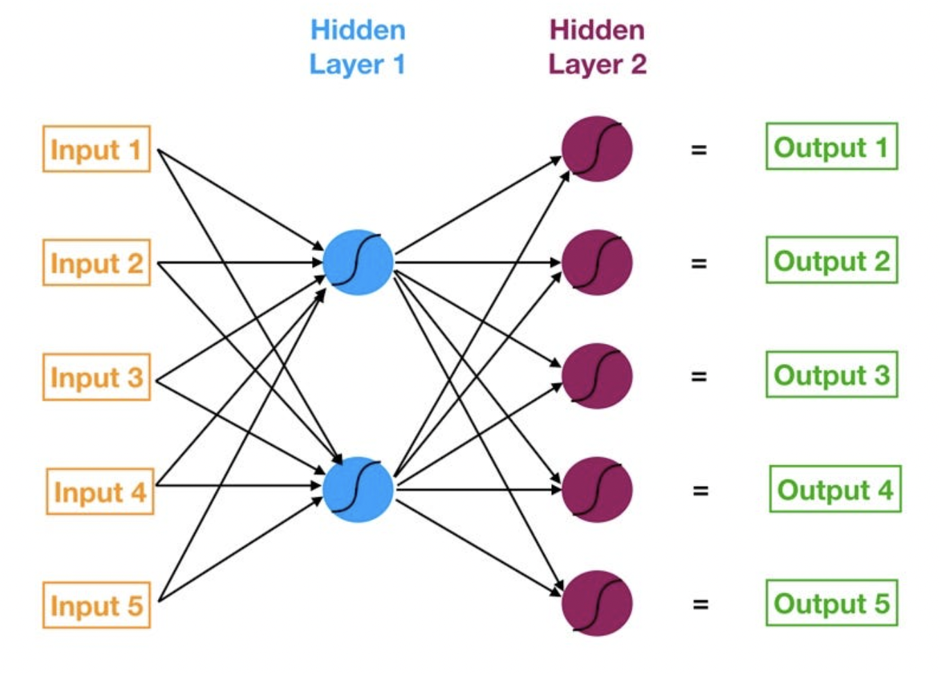
Neural Network Structure

Starting from the left, we have:

• The input layer of our model in orange.
• Our first hidden layer of neurons in blue.
• Our second hidden layer of neurons in magenta.
• The output layer (a.k.a. the prediction) of our model in green.
• The arrows that connect the dots shows how all the neurons are interconnected and how data travels from the input layer all the way through to the output layer.

2 - Information Propagation (Forward Pass)

2.1 - Linear Transformation $z = W \cdot X + b$

Each neuron computes a weighted sum of its inputs plus a bias term before applying an activation function.

2.2 - Activation Functions (ReLU, Sigmoid, Softmax)

Activation functions introduce non-linearity, enabling networks to learn complex patterns:

• ReLU: $f(z) = \max(0, z)$ (fast training, avoids vanishing gradients)
• Sigmoid: $\sigma(z) = \frac{1}{1 + e^{-z}}$ (useful for binary classification)
• Softmax: Converts outputs into probability distributions for multi-class classification.

3 - Learning and Backpropagation

3.1 - Cost Function (MSE, Cross-Entropy)

To measure error, different loss functions are used:

• Mean Squared Error (MSE): $$L(y, \hat{y}) = \frac{1}{n} \sum_{i=1}^{n} (y_i - \hat{y}_i)^2$$
• Cross-Entropy for classification: $$L(y, \hat{y}) = - \sum_{i=1}^{n} y_i \log(\hat{y}_i)$$

Where, $y$ represents the true values or labels, while $\hat{y}$represents the predicted values produced by the model. The goal is to minimize this difference during training.

3.2 - Gradient Descent and Weight Updates

Training consists of adjusting weights to minimize loss using gradient descent:

3.3 - Gradient Propagation via the Chain Rule

Using backpropagation, the error is propagated backward through the network using the chain rule, adjusting each weight accordingly.

4 - Optimization and Regularization

4.1 - Optimization Algorithms (SGD, Adam)

• Stochastic Gradient Descent (SGD): Updates weights after each sample.
• Adam: A more advanced optimizer that adapts learning rates per parameter.

The gradient of a function is the vector whose elements are its partial derivatives with respect to each parameter.So each element of the gradient tells us how the cost function would change if we applied a small change to that particular parameter – so we know what to tweak and by how much. To summarize, we can march towards the minimum by following these steps:

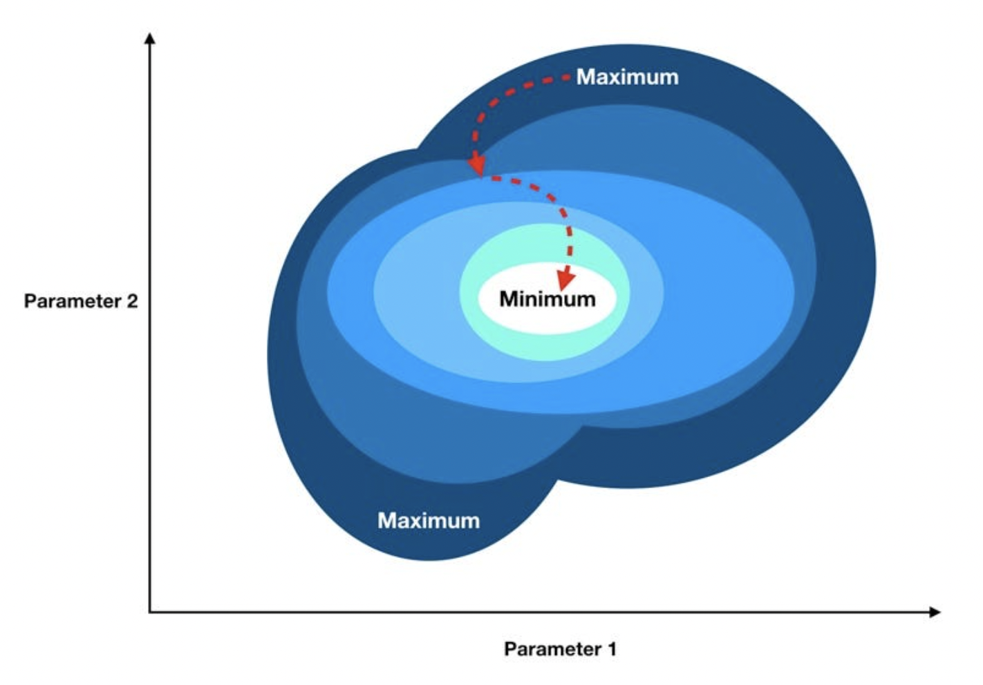
Gradient Descent

1. Compute the gradient of our "current location" (calculate the gradient using our current parameter values).
2. Modify each parameter by an amount proportional to its gradient element and in the opposite direction of its gradient element. For example, if the partial derivative of our cost function with respect to B0 is positive but tiny and the partial derivative with respect to B1 is negative and large, then we want to decrease B0 by a tiny amount and increase B1 by a large amount to lower our cost function.
3. Recompute the gradient using our new tweaked parameter values and repeat the previous steps until we arrive at the minimum.

4.2 - Regularization to Avoid Overfitting (Dropout, L1/L2)

To prevent overfitting:

• Dropout randomly disables neurons during training.
• L1/L2 regularization penalizes large weights to encourage simpler models.

5 - Network Architectures

Multi-Layer Perceptron (MLP) A standard feedforward neural network with multiple layers.

Convolutional Neural Networks (CNN) for Images Specialized for image processing using convolutional filters.

Recurrent Neural Networks (RNN, LSTM, GRU) for Sequences Useful for time series and natural language tasks.

Transformers for NLP and Vision State-of-the-art architecture for language understanding and vision tasks.

6 - Training and Evaluation

6.1 - Data Splitting (Train/Test Split)

To evaluate performance, data is split into training and test sets.

6.2 - Evaluation Metrics (Accuracy, Precision, Recall, RMSE, R²)

Metrics depend on the task:

• Accuracy, Precision, Recall for classification.
• RMSE, R² for regression.

6.3 - Hyperparameter Tuning

Choosing the right:

• Learning rate
• Batch size
• Number of layers and neurons

7 - Example: A Neural Network with Two Hidden Layers

The following example demonstrates a simple multi-layer perceptron (MLP) with two hidden layers, trained to perform linear regression.

import numpy as np
import tensorflow as tf
import matplotlib.pyplot as plt

# Generating data
X = np.linspace(-1, 1, 100).reshape(-1, 1)
y = 2 * X + 1 + 0.1 * np.random.randn(100, 1)  # y = 2x + 1 with noise

# Defining the model
model = tf.keras.Sequential([
    tf.keras.layers.Dense(10, input_shape=(1,), activation='relu'),  # First hidden layer
    tf.keras.layers.Dense(5, activation='relu'),  # Second hidden layer
    tf.keras.layers.Dense(1, activation='linear')  # Output layer
])

# Compiling the model
model.compile(optimizer='adam', loss='mse')

# Training the model
model.fit(X, y, epochs=200, verbose=0)

# Predictions
predictions = model.predict(X)

# Visualizing results
plt.scatter(X, y, label="Actual Data")
plt.plot(X, predictions, color='red', label="Model Predictions")
plt.legend()
plt.show()

8 - Conclusion

Neural networks form the foundation of modern artificial intelligence. Their ability to learn from data and generalize to new situations makes them essential for applications like computer vision, automatic translation, and predictive medicine. 🚀